Recognition and Visualization of Lithography Defects based on Transfer Learning

Research Article Archive • Versions 3 Vol 3 (3) : 20030302 2020

Bo Liu, Pengzheng Gao, Libin Zhang, Jiajin Zhang, Yuhong Zhao, Yayi Wei

DOI: 10.33079/jomm.20030302

： 2020 - 09 - 02

： 2020 - 09 - 28

： 2020 - 10 - 05

3281 23 0

Abstract & Keywords

Abstract: Yield control in the integrated circuit manufacturing process is very important, and defects are one of the main factors affecting chip yield. As the process control becomes more and more critical and the critical dimension becomes smaller and smaller, the identification and location of defects is particularly important. This paper uses a machine learning algorithm based on transfer learning and two fine-tuned neural network models to realize the autonomous recognition and classification of defects even the data set is small, which achieves 94.6% and 91.7% classification accuracy. The influence of network complexity on classification result is studied at the same time. This paper also establishes a visual display algorithm of defects, shows the process of extracting the deep-level features of the defective image by the network, and then analyze the defect features. Finally, the Gradient-weighted Class Activation Mapping technology is used to generate defect heat maps, which locate the defect positions and probability intensity effects. This paper greatly expands the application of transfer learning in the field of integrated circuit lithography defect recognition, and greatly improves the friendliness of defect display.

Keywords: transfer learning; neural network; lithography defects; visualize; Grad-CAM

1. Introduction

Defect reduction is particularly critical during the integrated circuit (IC) manufacturing process. At the lithography process stage, the rapid identification and correct classification of defects can help reduce the impact of defects and give a diagnostic result from the process. Defects are mostly caused by the environment, materials, processes, and so on, such as environmental airflow, the characteristic change of the materials, unreasonable changes of the equipment or incomplete cleaning steps, etc., which finally affect the process yield. Therefore, correct identification of defects and improvement of the accuracy and efficiency of defect identification are particularly critical for process control, and are also the key to competition with existing core equipment. In traditional lithography defect recognition, optical and electron microscopy imaging technologies are the most commonly used defect recognition technologies. It is based on image recognition technology to analyze and classify response signals. The size of defects that can be identified by optical measurement technology is relatively large, i.e. the level of micrometers and above. While electron microscopy imaging technology, such as the EBI or review machine, take the machine of ASML HMI for example ^[1], recognizes the defects by comparing different chip images. Through the continuous shrinking of the process, the defect control is becoming more and more stringent, which prompt engineers to use low-magnification and large field of view electronic scanning technology, and perform rapid comparison through spatial feature analysis ^[2]. The limitation of this method is that the types of defect cannot be automatically classified, and the size of the identifiable defect also be greatly restricted. Therefore, exploring a detection system that can quickly, efficiently and autonomously identify a variety of lithography defects is an important challenge for the yield of IC manufacturing.

At present, there have been many researches on the problem of lithography defect identification. In 2012, G. Luan ^[3]invented a method for identifying wafer defects using light sources and sensor devices. This device replaces the sensing unit of the sensor by judging the size of the crystal grain, so that the surface pattern of the crystal grain is correctly identified, thereby improving the accuracy of defect detection. In 2015, M. Wu and J. Chen et al. ^[4] used Support Vector Machine (SVM) algorithm to detect wafer defects under large-scale data set conditions, which significantly improved the defect recognition performance of the model. In 2019, D. Patel, R. Bonam et al. ^[5] aimed at line/space (L/S) structure defects, compared the fully connected layer and the global average pooling layer when constructing the Convolutional Neural Networks, analyzed the effects of the two output layer architectures on the recognition results, and realize the accurate and fast classification of L/S defects. So far, most of the related researches have used traditional image processing methods to identify large-scale defective images, and the procedures are complicated and cumbersome. Some of them use neural network to identify defects with small feature spans, which is relatively simple. It is rare to use transfer learning to identify multiple defects with a small-scale and a large feature span.

This paper carries out lithography defects detection based on transfer learning. By introducing two VGG Convolutional Neural Networks, autonomous analysis, feature extraction and data training will be carried out for defective image samples. By showing the visualized intermediate activation of the two networks ^[6], the process of extracting the deep-level features of the defective image are analyzed, which explores the learning mechanism of the network, and improve the classification accuracy. The use of Grad-CAM technology ^[7] achieves the autonomous rapid location of defects at the same time. This method will be used to improve the existing defect detection system in the field of IC manufacturing and improve the efficiency of autonomous identification.

2. Method

2.1. Transfer Learning and Convolutional Neural Networks (CNN)

Transfer learning ^[8] is a technology widely used in the field of image recognition. The advantage of this technology is that it can make full use of the pre-training model similar to the target task, and adjust the network structure and parameters through very few images to realize the rapid identification and recognition of defects classification. In the field of deep learning, it is impractical to use a small data set to train your own neural network from scratch. Due to the lack of data and too few learnable features, it usually leads to severe over-fitting (the performance of the model on the training set is much better than validation set and test set, which means a poor generalization ability). And transfer learning can solve this problem well through fine-tuning the general model that has been trained with a large data set, and then retraining a target model using the small data set.

The premise of transfer learning is to find a pre-trained neural network model similar to the target problem, and to modify the model parameters by limiting the training level and using a very small number of training images. In this paper, using a pre-trained CNN is very effective ^[9]. Pre-trained network has the characteristics of large original data sets and excellent performance on small data sets. And the CNN is a type of Feedforward Neural Networks with a deep structure whose main feature is convolution calculation. It has a clear structure and is suitable for transfer learning. In CNN, the two-dimensional convolution of the input image and the convolution kernel can be defined as:

(1)

In the formula, X represents the input image, W represents the convolution kernel, and

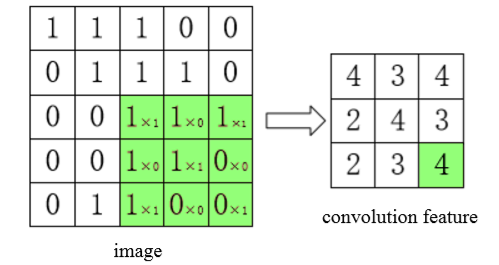
the right side of the equation represents the process of multiplying and adding the overlapping elements when the convolution kernel slides through the image ^[10]. As shown in Figure 1, when performing the convolution operation, the convolution kernel (green part) of size 3×3 slides through the image matrix of size 5×5 with a step length of 1, and the pixel values of the overlapping part are correspondingly multiplied and then added. Repeat this process until the entire image is traversed. Then, the convolution feature with the same size as the kernel can be obtained.

Figure 1. Example of convolution operation.

CNN has strong generalization ability, because it can allow the complexity of samples to a greater extent, and can well adapt to defective images with larger feature spans. CNN also has strong learning ability. For an image without any preprocessing, the network will extract the characteristic layer by layer, learn the effective features and send it to the solver to get the result. The biggest difference between CNN and traditional network is that the former has a negative feedback mechanism, which can realize the self-evaluation and improvement of the network during the weights update process.

2.2. Identification Algorithm

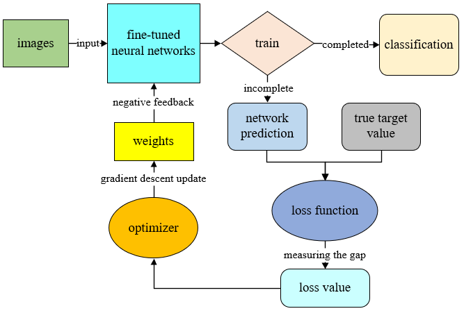
Figure 2. Working principle diagram of recognition algorithm.

Figure 2 illustrates the working principle flow of the recognition algorithm. With the fine-tuned neural network model, the overall realization principle of the recognition algorithm is as follows:

1. Input images into the fine-tuned neural network;

2. Calculate the network prediction value of the image for each class;

3. Use the loss function to measure the gap between the network predicted value and the true target value;

4. Pass this "gap" to the optimizer and update the network weights in the reverse direction;

5. Repeat the above operations until the network loss value is no longer decreasing;

6. Output the classification results.

2.2.1. The Structure and Working Principle of the Fine-Tuned Neural Network

The VGG16 and VGG19 ^[11] neural network models used in this study are both no-top structures, and the weights have been pre-trained on the large ImageNet data set for transfer learning.

Table 1. Comparison between fine-tuned VGG16 and VGG19 model structures.

Fine-tuned	Zero-padding	Number of layers Convolution	Max Pooling	GAP	Softmax
VGG16	13	13	5	1	1
VGG19	16	16	5	1	1

Table 1 shows the comparison between the fine-tuned VGG16 and VGG19 model structures, from left to right are the names of the network layers. It can be seen that the latter is higher than the former in terms of model complexity. Compared with other models, the VGG model have a clear structure and is more suitable for transfer learning of small data sets. Figure 3 shows the basic structure and working principle of the VGG model after the structure is fine-tuned. Each cube with a black border represents the feature maps of the image, and each cube with a green border represents the convolution kernel. First, use zero-padding at the edge of the input matrix to prevent the edge information of the image from being lost. Then use convolution kernel with a size of 3×3 to help the network obtain nonlinear features through convolution operations, and improve the model performance by deepening the number of network layers. The Max Pooling with a size of 2×2 and a stride of 2 is used to sequentially reduce the number of neurons after each convolution, which can not only achieve down-sampling and reduce computational costs, but also retain the salient features of the input image. After multiple convolution and max pooling iterations, the extracted last feature maps are connected to the Global Average Pooling (GAP) layer ^[12] to regularize the structure of the entire network to reduce the risk of over-fitting occurs. Finally, the GAP layer is connected to the Softmax Classifier ^[13] to realize the output of the predicted class of the input image.

Figure 3. Fine-tuned VGG neural networks.

2.2.2. Trainable Properties of the Fine-tuned Model

If the pre-trained network is directly used, the amount of network parameters are very large, and in the case of extremely limited training data set, it is difficult for the model to capture rich image features. The more training parameters, the greater the risk of overfitting. Usually before transfer learning, freezing layer is the basic operation of fine-tuned neural network^[14]. Freeze refers to setting the trainable of the layer to false. As the network fits the data, the weight remains unchanged. If the freezing operation is not performed before training, the features learned by the network will be modified due to the random initialization of the weights, and a large number of weight updates will be propagated in the network, which will cause great damage to the previously learned image features and affect the performance of the model. Therefore, freezing is essential in the fine-tuned process.

With the gradual deepening of the number of layers, the features extracted by the layers become more and more abstract. Layers closer to the bottom contain more information about image vision, so these layers encode more general reusable features; layers closer to the top contain more information about classification, so these layers encode more specialized features. Since this study needs to use a pre-trained network for the classification of defective images, the layers closer to the bottom of the fine-tuning will have less return, and the layers closer to the top are more useful to fine-tune. Therefore, this study only fine-tuning the last three convolutional layers and freezes the previous layers.

2.2.3 Optimization Algorithm of Neural Network

The core optimization algorithm of neural network is Backpropagation (BP). Because the neural network has too many layers, it is necessary to pass the network loss layer by layer from the output to the input through the BP algorithm, and update the network parameters in real time^[15]. This needs to pass the decreasing loss value to the optimizer, and update the weight of the network in the reverse direction, so that the network gradually optimizes its own performance, and then realizes the negative feedback of the network.

The specific principle of BP algorithm is gradient descent, so that the network loss value continuously converges to the global (or local) minimum. Since the gradient direction is the fastest direction in which the loss value increases, the negative gradient direction is the fastest direction in which the loss value decreases. Iterate step by step along the direction of the negative gradient to quickly converge to the minimum. This is the basic principle of the gradient descent method.

The loss function is a feedback signal used to learn the weight tensor. In the training phase, the smaller the loss value, the smaller the interval between the network predicted value and the true mark of the sample, and the stronger the model's ability to fit the data. It is an important indicator to measure the degree of match between the predicted value of the network and the true value. This model uses Cross Entropy Loss Function to calculate the cross-entropy loss through the probability output of the predicted class and the one-hot encoding of the true class. The function realization process can be expressed by the following:

(2)

In the formula, L represents the average of the loss value L_i of i samples, M represents the number of classes, y_ic is the symbolic variable (0 or 1, if the class is the same as the sample i, then 1 is taken, otherwise it is 0), p_ic represents the sample i belongs to the predicted probability of class c.

The optimizer used in this model is RMSprop, which has been proven to be an effective and practical deep learning network optimization algorithm. It combines the exponential moving average of the gradient square to adjust the change of the learning rate, thereby adaptively adjusting the gradient size in each direction, which can help the network to converge well when the loss function is unstable:

(3)

represents the weight at time t, α represents the learning rate, the default value is 0.001, g_t represents the gradient at time t, v_t represents the exponential moving average of the gradient square, \(\epsilon \) is a constant and the value is 10^-8 to avoid the divisor being 0.

Since the indicator is the ultimate manifestation of the model output purpose, and the model deals with is the classification problem, the indicator is classification accuracy.

2.3. Visualization Algorithm

The visualization algorithm includes visualizing the intermediate activation and the Gradient-weighted Class Activation Mapping (Grad-CAM). Visualizing the intermediate activation can eliminates the "black box" characteristics of the neural network, it helps to analyze which features of the defective image make the final classification decision. In the case of a classification error in the model, the decision-making process of the network can be debugged. Grad-CAM can realize the autonomous location of defects, which is of great significance for improving the automatic control system of integrated circuit manufacturing.

2.3.1. Visualizing the Intermediate Activation

Figure 4. Schematic diagram of visualizing the intermediate activation.

Visualizing the intermediate activation is to draw each channel of the output feature maps of the layers into a two-dimensional image, which is used to show the process of extracting the deep features of the defective image by the network^[16]. As shown in Figure 4, the image is input to the activation model based on the saved model. Then return the output to get the activation value of the middle layer of the saved model. Finally, post-processing can show the visualized intermediate activation.

2.3.2. Grad-CAM

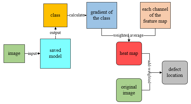
Figure 5. Grad-CAM principle diagram.

Grad-CAM can generate a heat map highlighting the focal area of the model for the output feature map of the network. As shown in Figure 5, the principle of Grad-CAM is: given an input image, for the output feature map of a convolutional layer, use the gradient of the class relative to the channel to weight each channel in the feature map, then calculate the channel-by-channel average value of the feature map to get the heat map. The weighted average method for a certain class of feature maps ^[7] can be expressed as:

(4)

(5)

c represents the output class,

represents the gradient of the class relative to the output feature map,

represents the mean gradient value of a particular feature map,

represents each channel of the feature map sample,

represents the channel-by-channel average value of the feature map, that is the heat map.

Use the add-weightedalgorithm ^[17] to calculate the sum of the corresponding values of each channel of the original image and the heat map to achieve defect location. The expression is:

(6)

dst represents the output location map matrix,

represents the pixel matrix of each channel of the original input image, and gamma represents the scalar value added to the sum of weights.

3. Experiment and Result Discussion

3.1. Data Collection, Analysis and Distribution

One of the main problems restricting the lithography process is the variety of defects. As shown in Figure 6, the lithography defects involved in this study include water pollution, collapse and residue.

Figure 6. Three types of lithography defects and defect-free images.

Water pollution is the main problem of the immersion lithography process. The remaining water stains will change the chemical sensitivity of the photoresist, cause degradation of the photoresist performance, and ultimately lead to local bridging. Collapse is caused by the surface tension of the water in the development process, which will cause large-area bridging. Residue is mainly caused by the incomplete cleaning step after the filter plate contact exposure during the photoresist etch-back process, and the light is completely blocked during the etching process of the wafer, which may cause missing or broken lines. According to the source of the defects, observe the image and analyze: the characteristic of water pollution is that the edge is diffuse and the shape is roughly elliptical; the characteristic of collapse is that the coverage area is large and the lines are sticky; and the characteristic of residue is that the edge is closed, distributed in blocks or dots. In this study, a comparison experiment was conducted on three types of defects by introducing defect-free images.

As shown in Table 2, the collected data is divided into training set, validation set and test set. The Training set will be used multiple times for feature extraction and data fitting, the validation set is used for the same number of times as the training set, preliminarily evaluate the performance of the model to determine whether the Training process has over-fitting, the test set is used only once to evaluate the generalization ability of the final model.

Table 2. Data distribution

	Water pollution	Collapse	Residue	Defect-free
Training set	68	64	34	109
Validation set	16	19	15	37
Test set	12	13	10	21
Total	96	96	59	167

3.2. Data Preprocessing

Data preprocessing is an indispensable work before model training, and a prerequisite to ensure smooth model training, including interference removal and data augmentation.

Interference removal part: Since the data sets are all SEM images, it is inevitable that there are measurement scales or light caused by human factors in the image. If there is interference in some data, other features that are irrelevant to the classification task will be extracted by the network, causing network fluctuations, and seriously affecting the performance of the model. Therefore, each sample image needs to be checked for interference. If interferences such as rulers and light spots are located at the edge of the image, these must be cropped; if the interference is inside the image, crop the largest size that does not include the interference.

Data augmentation part: Due to the limited data available, data augmentation of the training set images involves normalization, rotation, translation, horizontal flipping, random cross-cutting transformation and filling of newly created pixels. Normalization can compress the distribution value of image pixels from 0-255 to 0-1, which not only facilitates subsequent data processing, but also makes the convergence faster during network training. Rotation, translation, horizontal flip, random cross-cutting transformation, and filling of newly created pixels are data expansion of training samples. This process is implemented by Image Data Generator, which enables the model to observe richer image content. Since the data generated by this method is highly correlated with the original image, it cannot be used for validation data and test data.

3.3. Model Training, Validation and Testing

We use the training set to train two fine-tuned neural network models, the validation set to monitor the network fitting status, and the test set to evaluate the final performance of the model. The learning rate is adjusted to \({10}^{-5}\) after several attempts. The Early Stopping callback function is used to interrupt the current training when the validation accuracy is not improved for more than 10 rounds, and the Model Checkpoint callback function is used to not overwrite the model file when the validation loss is not improved, so that the network is always in best state.

3.3.1. VGG16

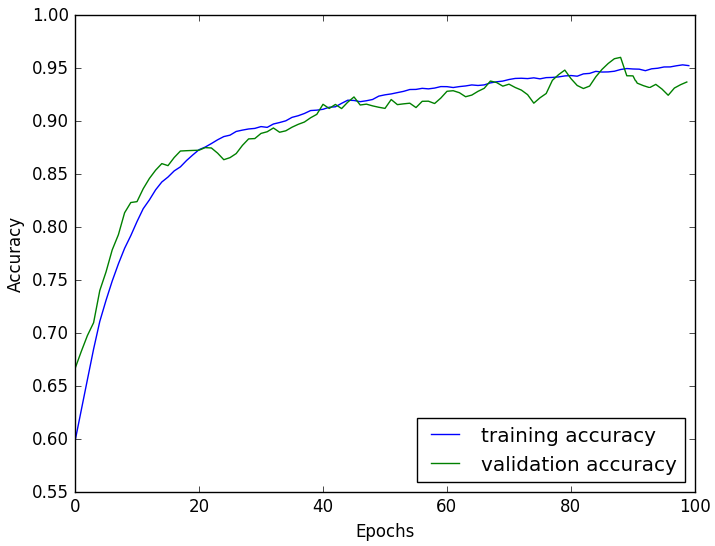
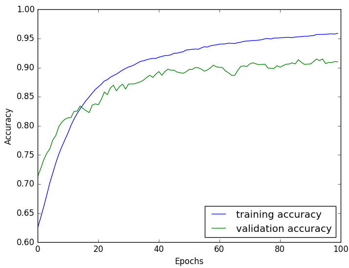
Figure 7. Evolution of training and validation accuracy with epochs for VGG16

Figure 7 shows the evolution of training and validation accuracy with epochs for VGG16 model. The horizontal axis represents the training epochs, the vertical axis represents the accuracy value, and the blue line and the green line respectively show the change trend of training accuracy and validation accuracy. Due to the use of more data augmentation in the training set, the data distribution has changed, resulting in the validation accuracy being slightly higher than the training accuracy in the early stage of training. The training and validation accuracy are almost monotonously improved, tending to be flat, and no over-fitting with the increase of epochs, indicates that the network is in continuous convergence.

Table 3. Confusion matrix of predicted and actual class under VGG16 model

Test set (N=56)		Water pollution	Actual Collapse	Residue	Defect-free
	Water pollution	11	1	0	1
Predicted	Collapse	0	12	0	0
	Residue	0	0	10	0
	Defect-free	1	0	0	20

Table 3 shows the performance of the VGG16 model on the test set in the form of a confusion matrix. As can be observed from this table, there is only two false negative and one false positive. We remind the readers that classification accuracy is the ratio of defective images that are being classiﬁed correctly to the total number of defective images, which is obtained by dividing the sum of diagonal elements by the total elements (94.6%).

3.3.2. VGG19

Figure 8. Evolution of training and validation accuracy with epochs for VGG19

Figure 8 shows the evolution of training and validation accuracy with epochs for VGG19 model. With the increase of epochs, the training accuracy is monotonously improving, while the validation accuracy increases rapidly at first, slowly in 20-40 epochs, and then stabilizes. Indicates that the network is fitted in advance. If continue to train, it will lead to over-fitting.

Table 4. Confusion matrix of predicted and actual class under VGG19 model

Test set (N=56)		Water pollution	Actual Collapse	Residue	Defect-free
	Water pollution	11	1	0	2
Predicted	Collapse	0	12	1	0
	Residue	0	0	9	0
	Defect-free	1	0	0	19

Table 4 shows the performance of the VGG16 model on the test set in the form of a confusion matrix. As can be observed from this table, there is three false negative and two false positive. The classification accuracy is obtained by dividing the sum of diagonal elements by the total elements, which is 91.7%.

It can be seen that although the training accuracy of the VGG19 model with more layers is slightly higher than that of VGG16, the validation and test accuracy of the former are not as good as the latter. It proves that the reason is caused by the relatively complex architecture of VGG19, which leads to poor adaptation to the lightweight data set. At the same time, we note that the false-negative images in both these models are the same types of images. We expect that by including more such images in our training dataset, our model might be able to pick that defect as well.

3.4. Visualization

3.4.1. Visualize Intermediate Activation

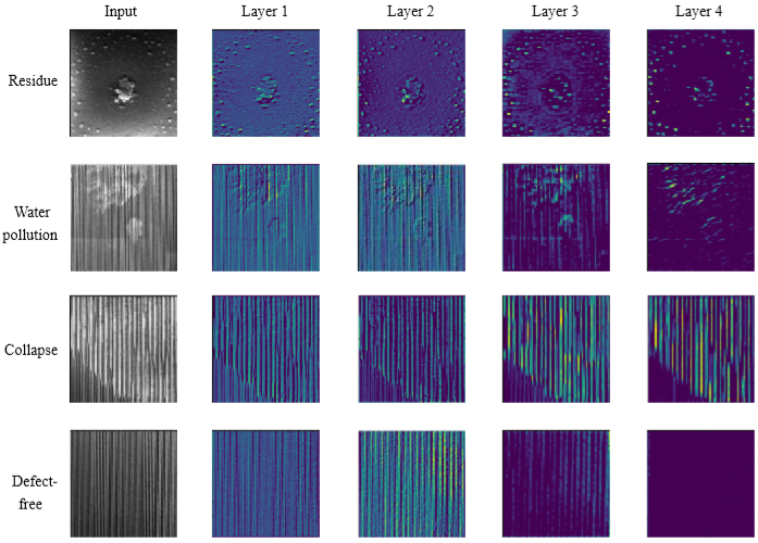
Figure 9. Visualized intermediate activation of the network

Figure 9 shows typical activation maps of four different classes of input images in the first four layers of the network. Layer 1 is a collection of various edge detectors. At this stage, activation almost retains all the information of the defective image. The function of Layer 2 is to highlight various useful feature information such as defect-specific block spots, textures, irregular lines, etc. to prepare for the feature extraction of the later layers. Layer 3 and 4 perform information distillation on the activation map of the previous layer, filter out useless information such as background patterns, regular lines, etc., enlarge and refine useful information. With the gradual deepening of the number of layers, the intermediate activation becomes abstract, contains less and less visual information and more and more abundant information of the class.

3.4.2. Defect Location

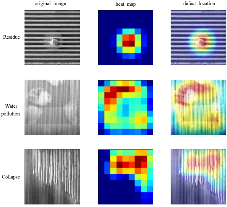
Figure 10. Defect location maps of the three classes

Figure 10 shows the original image, heat map and location map of the defects. The more obvious the defect is, the darker the color of the heat map display. After using the add-Weighted function to mix the original input image and the heat map, the heat distribution of the defect is added to the original image to achieve accurate positioning.

4. Conclusion

In this paper, we first demonstrated the recognition and classification of several lithography defects based on transfer learning. Through the training, validation and test of the two fine-tuned VGG16 and VGG19 neural network models, high classification accuracy (94.6% and 91.7%) of three types of defective images and defect-free images with a large feature span is achieved. Comparing the structural characteristics and classification results of the two models at the same time, it is found that the network with fewer layers and clearer structure is unlikely to occur over-fitting and has better performance when the data set is very small. It can be seen that the neural network model with fewer parameters has a better classification effect on lightweight data set.

This paper also analyzes which characteristics of the defects make the final classification decision by visualizing the intermediate activation of the network, and shows the process of the network gradually extracting the deep features of the defective images. Finally, the Grad-CAM technology is used to achieve rapid and accurate positioning of defects. Although it has not undergone explicit training, the model demonstrated remarkable defect recognition and location capabilities, proving its deployment potential in integrated circuit manufacturing.

Acknowledgments

Thanks for the support of the National Natural Science Foundation of China (61604172, 61874002) and the Key Laboratory of Microelectronic Devices and Integration Technology. The authors would like to thank Y. B. Feng from YMTC for the helpful discussions.

[1] J. Benschop, N. Harned, P. Kurz, “ASML program on EUVL: an update,” IEEE International Microprocesses and Nanotechnology Conference, 5037, 24-35 (2001).

+ CSCD · Baidu Scholar

[2] D.J. Friedman, M.H. Hansen, V.N. Nair, et al., “Model-free Estimation of Defect Clustering in Integrated Circuit Fabrication,” IEEE Transactions on Semiconductor Manufacturing, 10(3), 344-359 (1997).

+ CSCD · Baidu Scholar

[3] G. Luan, Wafer defect detection device and method, Worldwide applications, China (2012).

+ CSCD · Baidu Scholar

[4] M. Wu, J. R. Jang, J. Chen, “Wafer Map Failure Pattern Recognition and Similarity Ranking for Large-scale Data Sets”, IEEE Transactions on Semiconductor Manufacturing, 28(1), 1-12 (2015).

+ CSCD · Baidu Scholar

[5] D. Patel, R. Bonam, A. A. Oberai, "Engineering neural networks for improved defect detection and classification," Proc. SPIE10959 , 1095910 (2019).

+ CSCD · Baidu Scholar

[6] M. D. Zeiler, R. Fergus. “Visualizing and understanding convolutional networks[C]//European conference on computer vision,” Springer, Cham, 818-833 (2014).

+ CSCD · Baidu Scholar

[7] R. R. Selvaraju, M. Cogswell, A. Das, et al., "Grad-cam: Visual Explanations from Deep Networks via Gradient-based Localization," IEEE International Conference on Computer Vision, 618-626 (2017).

+ CSCD · Baidu Scholar

[8] S. J. Pan, Q. Yang, “A Survey on Transfer Learning,” IEEE Transactions on Knowledge and Data Engineering, 8(22), 1345-1359 (2010).

+ CSCD · Baidu Scholar

[9] P. Varalakshmi, G. Yuvaraj, K. Dhanasekaran, K. Samannan, "Diminishing fall-out and miss-rate in the classification of lung diseases using deep learning techniques," Tenth International Conference on, 373-376 (2018).

+ CSCD · Baidu Scholar

[10] M. Z. Zhang, V. K. Asari, "A Fully Pipelined Multiplierless Architecture for 2D Convolution with Quadrant Symmetric Kernels," IEEE Asia Pacific Conference on, 1559-1562 (2006).

+ CSCD · Baidu Scholar

[11] J. Sun, Z. Wu, Z. Yin, et al., "SVM-CNN-Based Fusion Algorithm for Vehicle Navigation Considering Atypical Observations," Signal Processing Letters IEEE, 26(2), 212-216 (2019).

+ CSCD · Baidu Scholar

[12] T. Y. Hsiao, Y. C. Chang, H. H. Chou, et al., “Filter-based deep-compression with global average pooling for convolutional networks,” Journal of Systems Architecture. 95, 9-18 (2019).

+ CSCD · Baidu Scholar

[13] Q. Rao, B. Yu, K. He, et al., “Regularization and Iterative Initialization of Softmax for Fast Training of Convolutional Neural Networks,” IEEE International Joint Conference on Neural Networks (IJCNN), 1-8 (2019).

+ CSCD · Baidu Scholar

[14] X. Liu, M. Chi, Y. Zhang, et al., “Classifying High Resolution Remote Sensing Images by Fine-Tuned VGG Deep Networks,” IEEE International Geoscience and Remote Sensing Symposium, 7137-7140 (2018).

+ CSCD · Baidu Scholar

[15] L. Pollini, M. Innocenti, “Improving on-line neural networks backpropagation convergence speed with mixed pattern-batch learning,” IEEE European Control Conference, 1282-1287 (1999).

+ CSCD · Baidu Scholar

[16] R. Sivaramakrishnan, S. Antani, Z. Xue, et al., “Visualizing abnormalities in chest radiographs through salient network activations in Deep Learning,” IEEE Life Sciences Conference, 71-74 (2017).

+ CSCD · Baidu Scholar

[17] R. Saha, K. D. Kim, “Add weighted algorithm based on the PICA and RBF neural network for image fusion,” International Conference on Electrical, Computer and Communication Engineering, 784-787 (2017).

+ CSCD · Baidu Scholar

Article and author information

Bo Liu

Pengzheng Gao

Libin Zhang

zhanglibin@ime.ac.cn

Jiajin Zhang

Yuhong Zhao

Yayi Wei

weiyayi@ime.ac.cn

Publication records

Published: Oct. 5, 2020 （Versions3）