Hotspot Detection of Semiconductor Lithography Circuits Based on Convolutional Neural Network

Research Article Archive • Versions 4 Vol 1 (2) : 18010205 2018

Xingyu Zhou, Youling Yu

DOI: 10.33079/jomm.18010205

： 2018 - 09 - 30

： 2018 - 12 - 27

3227 51 1

Abstract & Keywords

Abstract: In the advanced semiconductor lithography manufacturing process, the sub-wavelength lithography gap may cause lithographic error and the difference between the wafer pattern and mask pattern which may cause wafer defects in the later process. Even if a layout passes the design rule checking (DRC), it still might contain process hotspots which are sensitive to the lithographic process. Hence, process-hotspot detection has become a crucial issue. In this paper, we propose a convolutional neural network (CNN) based process-hotspot detection framework. Different network parameters including the training batch size, learning rate, loss functions as well as the optimization methods are compared and the optimal method is proposed with respect to a typical benchmark. The results of the tuned model are better than common machine learning methods. A general training flow is proposed. The method is flexible and can be applied to different benchmarks for better hotspot detection performance.

Keywords: lithography; hotspot detection; CNN; deep learning

1. Introduction

With the evolution of semiconductor technology nodes, the design of circuits is increasingly restricted by lithography conditions. Therefore, it is critical to verify the qualification of semiconductor design ^[1] from the perspective of lithography technology. The optical rule check method uses optical simulation to calculate the projected circuit pattern on a silicon wafer and finds the location of possible problems. Although the traditional optical simulation based circuit layout detection can identify most of the circuit areas that may lead to process defects, the uncertainty of the actual process conditions (photolithography, etching, etc.) and the rapid update of the process nodes make it harder for optical simulation based hotspot detection. Besides, the optical simulation requires a lot of computing resources. In order to make up for the lacking of optical simulations, geometric verification method ^[2] is proposed. This method has faster detection speed, because it only analyzes the layout itself and does not need to do complex optical simulation. Besides, pattern matching ^{[3, 4]}and some machine learning ^[5-8]methods have been tried. The pattern matching method is effective for the known hotspot detection which uses the known hotspot patterns in the template library to calculate its geometric similarity with the test layout. But it is difficult to detect unknown hotspots. Machine learning has the ability of supervised learning from known hotspot (HS) and non-hotspot (NHS) data sets. Because it can learn some hidden geometric features of the data sets during training, the model has the ability to detect unknown hotspots. Traditional machine learning methods are also accompanied with complex feature extraction and dimensionality reduction requirements. They may also suffer from a complicated framework. Some proposed methods show a high false positive ratio in the ICCAD2012 benchmark dataset ^[9].

In order to solve these problems, a hotspot detection method based on convolutional neural network is proposed in this paper. The layout of semiconductor circuits can be encoded to a numerical matrix as input which is suitable for the application of convolution neural networks ^{[10, 11]}. Convolution neural network can propagate the self-training of the convolution kernel, pooling kernel and full connection parameters by backpropagation. It can extract the hidden image features based on a certain network structure. We design a small network as a start. In order to further optimize the network and summarize the general training flow, this paper compares the influence of the batch size, learning rate, loss functions as well as optimization methods on the network performance, and does experiments on a set of benchmark data. Based on the simulation results, the optimized network parameters and learning method are recommended. A general optimization flow for model training is also proposed.

This paper describes the background of the problem in the second section. The third section introduces convolution neural network and software platform. In the fourth section, we introduce our network structure and the working flow. The fifth section shows the analytical results of the experiments. The last section summarizes the full text.

2. Problem Description

The problem of circuit hotspot detection ^[12] can be expressed as follows. Given a set of verified circuit layout with hotspot and non-hotspot labels, it is needed to build a model that can be used to identify unknown hotspots. The model should be able to increase the number of real hotspots detected and reduce the false detection rate.

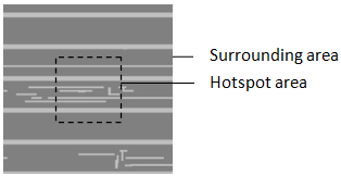
The circuit layout of the model input is shown in Figure 1. It includes the central hotspots and the related area that can be used to calculate the surrounding features. After training a model, we detect the layout of a testing circuit to determine which areas may contain hotspots. The trained model should detect the potential hotspots as far as possible. However, excessive detection will lead to overcompensation and false positive rate. Therefore, the model precision is also an evaluation indicator of the model.

Figure 1. Example of hotspot clip with surrounding area.

3. Algorithm and Software Platform

The convolution neural network (CNN) ^[13] is originally proposed to reduce the requirement of image data preprocessing and to solve the problem of image recognition. CNN can directly use image pixel information as input, reducing the process of many feature extraction. The most important feature of CNN is the weight sharing structure of convolution, which greatly reduces the parameters of neural network and restrains over-fitting. It has been widely used in the fields of Natural Language Processing, automatic driving, medical research and so on. This paper focuses on the application of convolution neural network in the field of industrial image recognition.

The Keras ^[14]framework used in this paper is a high-level neural network API, based on Tensorflow, Theano, and CNTK backends. Keras is highly modular, minimized, and scalable.

4. Framework of Hotspot Detection

4.1. Network Structure of Hotspot Detection Based on CNN

This paper builds the hotspot detection model based on CNN, and the network structure is shown in the Figure 2. The input layer is the normalized gray density value of image pixels. Each convolution layer contains a ReLU activation layer ^[15]. At the end of each convolution layer, there is a maximum pooling layer. Finally, all feature nodes are connected through the full connection layer and the classifier. The number of convolution, pooling, and full connection layers can be manually adjusted according to specific problem. At the same time, the over fitting of the network should be avoided. We can judge when to stop training observing performance of cross validation set. Adding parameter regularization term and drop out will also help. This paper aims to research the influence of training parameters and learning methods on hotspot detection performance instead of the layer structures. Therefore, we use the following network structure as shown in Figure 2.

Figure 2. Hotspot detection network structure based on CNN.

In this paper, we use the gray density of image pixels as the input of the whole neural network. We use a 5×5 convolution kernel to extract different features of image. And the input image is supplemented of two zero layers. The parameters of each convolution unit are optimized by backpropagation algorithm.

The activation function adds nonlinear factors to the network. Commonly used activation functions are sigmoid functions, tanh functions, and ReLU functions^[15]. ReLU function and its derivative are used in this paper. The performance of ReLU activation function highly depends on an appropriate learning rate.

Pooling is another important concept in convolutional neural networks. It is actually a form of sampling reduction. There are many different forms of nonlinear pooling functions, of which "Max pooling" is the most common. It divides the input image into several rectangular regions and outputs the maximum value for each sub-region. Pooling layer will continuously reduce the size of the data space, so the number of parameters and the amount of calculation will also decline, which to a certain extent controls the over-fitting and improves the generalization ability of the model.

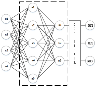
The convolution layer, pooling layer and activation function layer are used to map the original data to hidden feature space while the full connection layer plays a role of feature weighting. Different networks may contain different depths of full connection layers. Generally, increasing the number of layers is usually helpful to increase the accuracy of classification, but too many layers will lead to over-fitting which causes the classification effect of verification set to decline. The full connection layer is shown in Figure 3.

Figure 3. Full connection layer.

Output layer also known as the loss function layer is used to determine how the training process "punishes" the difference between the predicted and actual results of the network, which is usually the last layer of the network.

4.2. Hotspot Detection Process Based on CNN

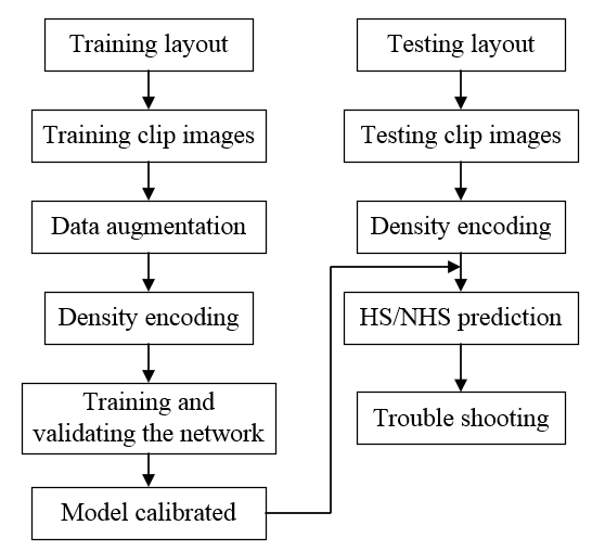
As shown in Figure 4, after the image augmentation and graphic encoding, the training classifier model is trained by adjusting the training scale, learning rate, loss function, learning method and other factors. When the recognition results of the verification set meet the requirement, the model is applied to the testing set to evaluate the model performance.

Figure 4. Hotspot detection process based on CNN.

Because of the unbalance between the data set, hotspot samples need to be augmented before training. In this experiment, the horizontal and vertical inversion augmentation method is used.

The training process can be introduced as two main parts which are the forward propagation and back propagation.

4.3. Forward Propagation

1) Collect the labeled images and convert them to 172×172 pixel normalized grayscale images. Randomly pick 60% of the labeled images as training set, and the left as cross validation set.

2) Convolute the input images as Function 1 and activate them by Relu activation function as Function 2.

(1)

(2)

3) Extract the local maximum of the pooling region by maximum pooling layer as Function 3 to reduce the spatial size of the data and increase the robustness of the network.

(3)

4) Repeat step 2 and 3 while the number of convolution filters, the size of convolution kernel, the size of pool kernel and the step size of each layer can be adjusted.

5) Stretch the image matrix from the final pooling output into a one-dimensional vector as the input of the full-connection layer. The full-connection function is given as

(4)

6) Take the image information of the last hidden layer as input. The Squared_hinge (sh) loss function is as Function 5 where

is 1 or -1. The softmax and Categorical_crossentropy (cc) loss functions are as Function 6-7 where

is 1 or 0 and

stands for the probability that an image

belongs to category

(5)

(6)

(7)

4.4. Back Propagation

1) For Squared_hinge classifier, the back propagation is as Function 8. For Categorical_crossentropy classifier, the back propagation is as Function 9-10.

stands for total categories and

stands for number of samples. The difference of them will be compared later in this paper.

(8)

(9)

(10)

2) The back propagation of the full connection layer is given as Function 11-14 where

is the loss of the full connection layer.

(11)

(12)

(13)

(14)

3) The backpropagation of the pooling layer is as Function 15.

(15)

4) The backpropagation of the convolution layer is as Function 16-18.

(16)

(17)

(18)

5. Experimental Results and Analysis

5.1. Training and Validation Results

This paper uses the data sets of ICCAD to train and verify the designed network. The details are as Table 1.

Table 1. ICCAD data sets.

Dataset	Train		Test		Process
Dataset	#HS	#NHS	#HS	#NHS	Process
ICCAD-1	99	340	226	319	32nm
ICCAD-2	174	5285	499	4146	28nm
ICCAD-3	909	4643	1847	3541	28nm
ICCAD-4	95	4452	192	3386	28nm
ICCAD-5	26	2716	42	2111	28nm

All training sets are divided into 3:2 for training and cross validation. The effects of different batch sizes, learning rate, loss function and optimization methods are analyzed and compared. The differences of every result are explained. After four experiments, the precision and recall of the best model are tested on testing set.

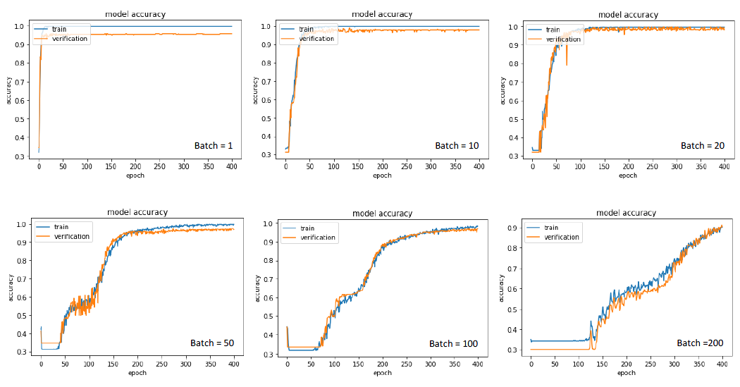
Experiment 1 analyzed the effect of training batch^[16] on the model. Keep the learning rate, loss function and optimization method unchanged. Training results of ICCAD-1 data set are as Figure 5. Increasing batch size within a certain range can improve memory utilization and reduce the number of iterations every epoch. Usually, the greater the batch size, the more accurate the gradient descent direction is, and the smaller the training vibration. But too large batch size has the problems of memory overflow, slow convergence and local optimum. Therefore, we need to consider the size of batch size based on factors such as time, memory space and accuracy. For ICCAD-1 data set, batch size 20 is reasonable to have a high validation accuracy and appropriate computing time.

Figure 5. Effects of the batch size on model accuracy.

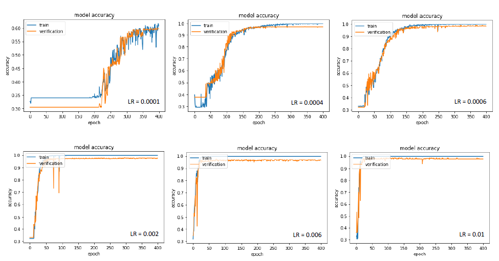
Experiment 2 analyzed the effects of Mini-batch Gradient Descent (MGD) learning rate (LR)^[17] on the model. Keep the batch size, loss function, and optimization method unchanged, and adjust the learning rate. Experimental results are as Figure 6. It is proved that too large learning rate leads to an over update which makes the model difficult to converge. In addition, because the activation function is ReLU, too large learning rate will make many nodes turn to 0 after iterations of activation functions and the gradient will stop to decline. In this experiment, when the learning rate is under 0.01, the model can converge and the accuracy is acceptable. And the smaller learning rate needs more iterations to achieve convergence. Training time also increases correspondingly. It is remarkable that too small learning rate is not only time consuming but also could cause local optimum. Therefore, the choice of learning rate should be considered taking the accuracy, training time, and optimization methods into account.

Figure 6. Effects of learning rate on model accuracy.

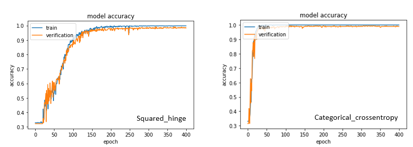
Experiment 3 analyzed the effects of loss function^[18] on the model. Keep the batch size, learning rate, and optimization method unchanged, and adjust the loss function. Training results of data set ICCAD-1 are as Figure 7. Squared_hinge is a classification method based on the maximum boundary. It maximizes the minimum distance between the classification surface and the feature vector to optimize the model. It focuses on the features near the classification surface. Categorical_crossentropy is a classifier based on probability distribution, which reduces the probability of misclassification by cross entropy function and pays attention to all features. We can see that the two loss functions both converge well, and the Squared_hinge’s convergence speed is slower, which is related to the features of the training set. Considering the explanatory property and robustness of the classification model, the Categorical_crossentropy is chosen as the loss function in this paper.

Figure 7. Effects of the loss function on model accuracy.

Experiment 4 analyzed the effects of optimization methods^[19] on training results. Keep the batch size, initial learning rate, and loss function unchanged, and adjust the optimization method. The experimental results are as Figure 8. MGD is the most common optimization method which calculates the gradient of mini-batch every iteration and then updates the parameters with the same learning rate. The choice of learning rate will directly affect the performance of optimization. Adagrad imposes a constraint on the learning rate. It increases the learning rate of more sparse parameters and decreases the learning rate of parameters which upgrades faster in the past. However, Adagrad has a problem of early stop when training a deep network because of its monotonic adjusting strategy. While Adagrad accumulates all the squares of the gradient before calculating the corresponding learning rate, Adadelta adapts learning rates based on a moving window of gradient updates. It is shown that the adaptive learning methods converge more quickly which doesn’t need a careful design of the initial learning rate. Adadelta is chosen as the final optimization method for its learning speed and robustness. It is worth mentioning that MGD is still widely used nowadays for its final tune ability and flexibility for researching.

Figure 8. Effects of the optimization method on model accuracy.

5.2. Testing Results

The recall and precision are defined as Function 19-20. #Hit means the number of detected real hotspots. #HS means the total hotspots in testing set. #Extra means the number of wrongly detected hot spots.

(19)

(20)

As introduced above, setting batch size to be 20, using Categorical_crossentropy as the loss function and Adadelta as the optimization method, the testing results of the ICCAD testing sets are as Table 2. Though the network is not deep, the performance is better than SVM-based methods in all categories mainly because of the hidden neural network which is good at finding non-linear relations and the probability based loss function which takes all the features of samples into account. The adaptive optimization method also contributes.

Table 2. Testing results

Test layout	Methods	Recall	Precision
ICCAD-1	This	0.963	0.310
	B. Yu^[20]	0.810	0.202
	Y. T. Yu^[21]	0.947	0.125
ICCAD-2	This	0.996	0.180
	B. Yu^[20]	0.811	0.039
	Y. T. Yu^[21]	0.982	0.040
ICCAD-3	This	0.987	0.194
	B. Yu^[20]	0.909	0.089
	Y. T. Yu^[21]	0.919	0.109
ICCAD-4	This	0.980	0.082
	B. Yu^[20]	0.870	0.054
	Y. T. Yu^21]	0.859	0.043
ICCAD-5	This	0.972	0.067
	B. Yu^[20]	0.805	0.047
	Y. T. Yu^[21]	0.929	0.031
Average	This	0.980	0.167
	B. Yu^[20]	0.841	0.086
	Y. T. Yu^[21]	0.927	0.070

6. Conclusion

In this paper, the convolutional neural network theory is applied to the lithography circuit pattern inspection. Principles of CNN are introduced. The effects of different network parameters and learning methods on the model are analyzed and compared. The final proposed model has a nice performance on the testing set with respect to precision and recall. CNN can solve many problems. The optimal network parameters and learning methods can vary according to different applications. But the process of training model is consistent. This paper gives a hint for advanced patterning solutions and also provides a reference for researchers who want to improve the network performance.

[1] D. Z. Pan, B. Yu, and J. R. Gao, “Design for manufacturing with emerging nanolithography,” IEEE Trans. Comput. Aided Des. Integr. Circuits Syst. 32 (10), 1453-1472 (2013).

+ CSCD · Baidu Scholar

[2] Y. T. Yu, Y. C. Chan, S. Sinha, I. H. R. Jiang, and C. Chiang, “Accurate process-hotspot detection using critical design rule extraction,” Proc. 49th Annu. Des. Autom. Conf., 1167-1172 (2012).

+ CSCD · Baidu Scholar

[3] Z. Xiao, Y. Du, H. Tian, et al., “Directed self-assembly (DSA) template pattern verification,” Proc. DAC, 55:1-55:6 (2014).

+ CSCD · Baidu Scholar

[4] W. Y. Wen, J. C. Li, S.Y. Lin, et al., “A fuzzy-matching model with grid reduction for lithography hotspot detection,” IEEE Trans. Comput. Aided Des. Integr. Circuits Syst.33 (11), 1671–1680 (2014).

+ CSCD · Baidu Scholar

[5] T Matsunawa, J. R. Gao, B. Yu, et al., “A new lithography hotspot detection framework based on AdaBoost classifier and simplified feature extraction,” Proc. SPIE 9427 , 94270S (2015).

+ CSCD · Baidu Scholar

[6] Z. Sun, F. Li, H. Huang. “Large Scale Image Classification Based on CNN and Parallel SVM,” Neural Information Processing, 545-555 (2017).

+ CSCD · Baidu Scholar

[7] D. Ding, A. J. Torres, F. G. Pikus, and D. Z. Pan, “High performance lithographic hotspot detection using hierarchically refined machine learning,” Proc. Asia South Pac. Design Autom. Conf. (ASP-DAC), 775-780 (2011).

+ CSCD · Baidu Scholar

[8] D. Ding, J. A. Torres,D. Z. Pan , “High Performance Lithography Hotspot Detection With successively Refined Pattern Identifications and Machine Learning” Computer-Aided Design of Integrated Circuits and Systems, IEEE Press, 1621-1634 (2011).

+ CSCD · Baidu Scholar

[9] J. A. Torres, “ICCAD-2012 CAD contest in fuzzy pattern matching for physical verification and bench mark suite,” Proc. Int. Conf. Comput. Aided Des. (ICCAD) 349-350 (2012).

+ CSCD · Baidu Scholar

[10] N. Nagase, K. Suzuki,, K. Takahashi, M. Minemura, S. Yamauchi, and T. Okada, “Study of hot spot detection using neural network judgment," Proc. SPIE6607 , 66071B (2007).

+ CSCD · Baidu Scholar

[11] K. Simonyan, A. Zisserman, “Very deep convolutional networks for large-scale image recognition,” arXiv preprint (2014).

+ CSCD · Baidu Scholar

[12] J. R. Gao, B. Yu, D. Z. Pan, “Accurate lithography hotspot detection based on PCA-SVM classifier with hierarchical data clustering,” J. Micro/Nanolith. MEMS MOEMS14 (1), 2006-2021 (2014).

+ CSCD · Baidu Scholar

[13] S. Chaib, H. Yao, Y. Gu, et al., “Deep feature extraction and combination for remote sensing image classification based on pre-trained CNN models,” Int. Conf. Digital Image Processing (ICDIP)10420 , 104203D (2017).

+ CSCD · Baidu Scholar

[14] Keras: The Python Deep Learning library. Available: https://keras.io.

+ CSCD · Baidu Scholar

[15] Y. Lavinia, HH. Vo, A. Verma, “Fusion Based Deep CNN for Improved Large-Scale Image Action Recognition,” IEEE Int. Sympo. Multimedia, 609-614 (2017).

+ CSCD · Baidu Scholar

[16] C. Peng, T. Xiao, Z. Li, et al., “MegDet: A Large Mini-Batch Object Detector,” arXiv (2017).

+ CSCD · Baidu Scholar

[17] R. Zhan, J. Hu, J. Zhang, “Adaptive learning rate CNN for SAR ATR,” Cie Int. Conf. Radar, 1-5 (2016).

+ CSCD · Baidu Scholar

[18] C. Y. Lee, S. Xie, P. Gallagher, et al., “Deeply-Supervised Nets,” arXiv, 562-570 (2014).

+ CSCD · Baidu Scholar

[19] P. Johnbaptiste, E. Zelnio, G. E. Smith, “Using deep learning for SAR image optimization,” Proc. SPIE10647 , 106470D (2018).

+ CSCD · Baidu Scholar

[20] B. Yu, J. R. Gao, D. Ding, X. Zeng, and D. Z. Pan, “Accurate lithography hotspot detection based on principal component analysis-support vector machine classifier with hierarchical data clustering,” J. Micro/Nanolith. MEMS MOEMS14 (1), 1-12 (2014).

+ CSCD · Baidu Scholar

[21] Y. T. Yu, G. H. Lin, I. H. R. Jiang, and C. Chiang, “Machine-learning-based hotspot detection using topological classification and critical feature extraction,” Proc. 50th Annu. Des. Autom. Conf., 671-676 (2013).

+ CSCD · Baidu Scholar

Article and author information

Xingyu Zhou

Youling Yu

Publication records

Published: Dec. 27, 2018 （Versions4）