Since the quasi Fermi potentials Φ
n and Φ
p (imrefs) for electrons or holes, respectively, cover a much smaller range of numerical values compared to the electron or hole densities
n,
p, intermediate and final solutions of the drift diffusion system of equations are typically saved by storing the electrostatic potential Ψ, and the imrefs Φ
n and Φ
p instead of Ψ,
n and
p. Moreover, formulating the DD equations in Ψ, Φ
n, and Φ
p makes it much easier to introduce the solution algorithms that are typically applied. The stationary drift diffusion equations for a homogeneous semiconductor (e.g., silicon) device formulated in these variables have the following form (see References [
7, 4,
8,
9] for details and a derivation),


(1)

(2)

(3)
where e is the elementary charge and κ is the permittivity of the different materials for which Poisson’s Equation (1) is solved. Moreover ni is the intrinsic density, ND , NA are the ionized donor and acceptor concentrations and µn , µp the electron and hole mobilities of the semiconductor material with homogeneous band gap within which the electron and hole continuity Equations (3, 2) are solved. In addition, VT is the thermal voltage and G the generation density within the semiconductor. For simplicity it is assumed that at all contacts the Dirichlet boundary conditions of the ideal Ohmic contact model (see References [4, 9] for details) are valid for all three potentials Ψ, Φn and Φp and that at all other boundaries homogeneous Neuman type boundary conditions can be applied.
It can be shown that the above system of differential equations has a unique solution provided a number of reasonable assumptions is fulfilled especially for the generation term G. Please refer to Reference [
10] for a general theory and to References [
11,
12] for special results concerning the DD set of equations.
There is an important property, that deserves special attention.
I. All above operators TP - TE are in divergence form and result in important conservation laws if integrated over a finite volume and after the application of the divergence theorem.
For example integrating TH+TE over the simulation domain results in Kirchhoff’s law for the stationary terminal currents of the device under consideration. If a numerical device model is used inside a circuit simulator it is absolutely mandatory that this law is exactly reproduced by the numerical model. Therefore, it is very important to maintain the validity of such conservation laws in some sense during the discretization process.
The most important solution algorithm for the DD system is an iterative method often addressed as Gummel’s nonlinear relaxation method [1]. Assuming the result Ψk, Φp,k, Φn,k, after iteration k as known, this method evaluates the new approximate solution after iteration k+1 by solving the three boundary value problems (1) - (3) successively as follows:

(4)
For the above partiell differential equations it is always assumed that the variable with the highest number of derivatives in the equation is updated and the other variables are kept unchanged. The individual nonlinear equations in (4) are typically solved by Newton’s method, which converges very fast and robust even for bad initial solutions, if the underlying equation is nearly linear. Therefore, Newton’s method is typically applied for the operators

and

defined in (2) and (3) and not for the operators
TH and
TE, since

and

are nearly linear in the new variables

(5)
provided carrier generation G has no dominant influence. These new variables are often addressed as Slotboom variables because they were first introduced in Reference [
13] and the advantages they have for generating “stable” discretization schemes were probably mentioned in Reference [7] for the first time. Nevertheless it is still possible to calculate the Newton updates based on the numerically more convenient Jacobians of
TH and
TE and the variables Φ
p and Φ
n. The only modification necessary for performing the Newton iterations for the more linear operators is to modify the Newton update itself as shown below for the hole continuity equation and the solution function before (Φ
p,b) and after (Φ
p,a) one Newton step.

(6)

is the Newton update calculated using the Jacobian of
TH for the variable

. For a general report on using alternative solution variables for enhancing convergence please refer to Reference [
14].
In order to understand which criteria in addition to the mandatory consistency criterion should be considered for the discretization of the continuous operators
TP -
TE it is very useful to look at the Jacobians of

,

and

that are necessary for performing Gummel’s nonlinear relaxation method based on Newton’s method. These Jacobians are typically evaluated for some existing intermediate solution Ψ
b, Φ
p,b, Φ
n,b and operate on the functions

,

,

. If in addition for the calculation of the Jacobians the dependence of the mobilities on the solution variables is neglected,
these Jacobians have the following form.:

(7)

(8)

(9)
All above partial derivatives with respect to solution variables are assumed to be Frechet derivatives on suitable function spaces
[15]. If only direct recombination and Shockley-Read-Hall (SRH) recombination
[9] is considered for the Frechet derivative of the carrier generation G

(10)
holds. With this additional condition all Jacobians (7)-(9) have important properties that again deserve special attention. They are
II. self adjoint,
III. positive definite,
IV. of monotone typ,
if appropriate boundary conditions are assumed for the function spaces considered
[15]. Especially property IV is very important, since it means that for all these Jacobians monotonicity theorems hold (Reference [15], Chapter 23.5) which restrict for example the possible form of the update functions

,

,

during the Newton iterations required for Gummel’s nonlinear relaxation method very much and enhance the robustness and convergence properties of this solution method decisively.
The mathematical properties of the model after discretization should be as similar as possible to the properties of the continuous model! If this is fulfilled the discrete model is an analogon of the continuous model, even if only coarse grids can be afforded, which is typically the case. This property is very important for the discretization error control on coarse grids. Therefore discretization methods are preferred which are able to conserve conditions I-IV in some discrete sense.
The first 2D DD simulations used a rectangular solution domain and tensor product grids
[16, 7] so that standard finite difference discretization methods for tensor product grids could be applied, that conserved most of the conditions mentioned above. However many device cross sections were not rectangular, so that at least at the beginning of multi-dimensional numerical semiconductor device modeling many groups developed discretization methods (see References [
17,
18,
19,
20, 5,
21,
22] and citations therein) for non rectangular solution domains based on the finite element approach
[23], but it turned out that general finite element methods typically have problems to conserve conditions I-IV
[24, 18, 5, 25]. Finally, even for solution domains with complicated polygonal boundaries which cannot be discretized efficiently by a tensor product grid, the method of choice used today by the vast majority of DD and HD simulators is a straight forward generalization of the integration method published in Reference [26], Chapter 6 for 2D tensor product grids. This method is able to conserve conditions I-IV as will be shown below. This generalization for 2D problems was already briefly mentioned in Reference [
26] using the early work of Reference [
27] as guideline. This general method is addressed as box integration method in Reference [4], as box method in Reference [5] and today often named finite volume method
[28]. An especially well documented example of this historical development from the application of general finite element methods to the final exclusive application of the finite volume method is the development of numerical device modeling codes at IBM research. There two groups independently developed two general numerical device modeling codes. One group with a clear focus on the application of general finite element methods
[24, 19, 20] and the other group shifting more and more from hybrid finite element/ finite volume discretization methods to the exclusive application of the finite volume method
[29, 18]. Both codes were developed over a decade until the beginning of the eighties. Ten years later the finite element code development is not mentioned at all any more in a comprehensive review paper about the TCAD development at IBM with more than 200 citations
[30].
Possibly the first mathematical analysis of the general box integration method for the DD model in 3D is due to Reference [
31]. The box integration method can be interpreted as a finite element method
[5], but the grid elements for this method (e.g. triangles) cannot be considered as the basis from which the discretization method proceeds like it is the case for a general finite element method
[23] but instead the elements are constructed in a unique way based on the predefined grid points. The method is based on the construction of two dual grids the Voronoi diagram and the Delaunay tessellation. The early work of the two Russian mathematicions M.G. Voronoi
[32] and B.N. Delone
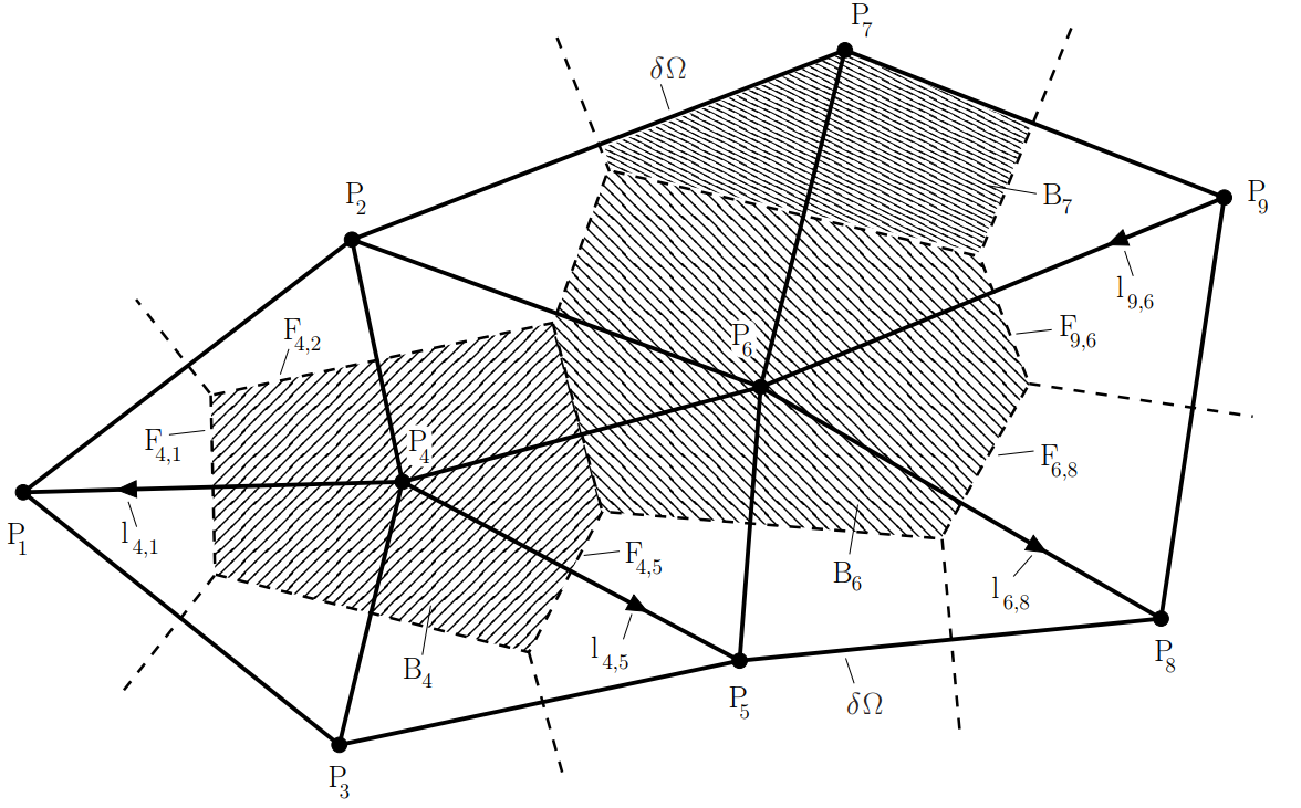
[33] is typically cited in this context but the method in 2D is even much older and has been rediscovered various times. Figure 1 below is used to explain the basic principles of this method. The n grid points
Pk (
n = 9 in this example) with the coordinates

are considered as given. In a first step for each point with index
k its Voronoi volume
Vk is constructed as the set of all points in space that are closer to
Pk than to any other grid point.

(11)
Moreover for each grid point Pk its environment Sk is defined by

(12)
M indicates the 1D Lebesgue measure M1 for 2D problems and the 2D Lebesgue measure M2 for 3D problems. With this environment the boundary of Vk is given by

(13)
Figure 1.
Voronoi diagram (dashed lines) and Delaunay tessellation (thick drawn lines) for a 2D example with 9 grid points. The union of all Voronoi volume boundaries defines the Voronoi diagram. Based on this diagram the dual grid structure of the Delaunay grid is defined by defining the set of edges D for this grid by the straight lines
li ,k between the points P
i and P
k for which

and
i and
k vary between 1 and
n with

. Please note that the
li ,k are oriented curves starting at P
i and ending at P
k. If only the edges of the Delaunay grid without orientation are important
li ,k and
lk ,i can be considered as equal. The typical elements in such a Delaunay grid for 2D problems are triangles and tetrahedra for 3D problems. But 2D and 3D rectangular tensor product grids are special cases for this method and fit perfectly into this framework. The DD and HD problems are typically formulated as boundary value problems on some finite region

and in order to incorporate Newman type boundary conditions into the framework of box integration in a natural manner the boundary

is typically assumed to be composed of edges (faces in 3D) of the delaunay grid elements. In the given example in Figure 1,

is the closed polygonal line composed of

,

,

,

,

,

and

and
is the interior of this closed polygonal line. The Voronoi volumes for the grid points on
are typically unbounded but for box integration bounded boxes are mandatory. This leads to the following definitions:

(14)

(15)
Clearly

and

is only relevant if

is part of the Delaunay grid. If no additional constraints are fulfilled it can happen that

for some edge of the Delaunay grid. This is typically not good for the consistency of the discretization method and mostly avoided by constructing the grid in such a manner that for example for 2D problems like the given example the Delaunay triangles that have some common boundary edge with
have all interior angles smaller than 90 degrees. Such triangles are called acute or nonobtuse. See for example Reference [
34] for algorithms generating grids in such a manner. If this additional condition is fulfilled

for all edges of the Delaunay grid holds and only the boxes

of grid points on the boundary
share some boundary with
like

for the given example. Similar additional conditions with comparable consequences are considered as well for 3D problems
[31]. For the box integration process presented here it is not necessary that all triangles are nonobtuse for preserving condition IV but for finite element discretization schemes this condition must be fulfilled
[34, 5].
The boundary value problems
TP,

and

defined in Equations (1) - (3) and considered as individual problems that are solved separately have the following common form:

(16)
u (
r) is the solution variable. Therefore
u is either

or

or

. Morover

holds always. The dependence of
a and
f on

and
u considers the typical physical models for the mobilities and the generation rate and their dependence on the solution variables
[9]. The first step always performed for the box method is to integrate Equation (16) over the box

for each grid point

, which is not determined by a Dirichlet boundary condition. Moreover the divergence theorem is used to transform the suitable parts of the integral over
into integrals over

. This yields:

(17)

is a unit vector having the same orientation as

. The above formulation is for the 3D case, where the first integrals integrate fluxes over an area and the remaining part is a volume integral. In the 2D case the first integrals are line integrals and the second part is an area integral. If

it can typically be assumed that for this part of the boundary

a Newman type boundary condition holds such that the flux through this part of the boundary is zero. This applies for instance for

in the example, if for

no Dirichlet boundary condition is given. It is clear that

(18)
where the first integral is related to

and the box integration over

, whereas the second integral is related to the point

and the box integration over

. During the discretization process the integrals in Equation (17) are typically approximated independently by difference approximations and quadrature rules such that a consistent discrete approximation is generated. For conserving property
I it is important that Equation (18) holds exactly after discretization. If this is the case the discretized formulas for two points
and
with

(like

and

in the example) can be summed leading to an expression where the sum of the discretized integrals over
and

is represented by the discretized flux integrals over the boundary of

which is

. The resulting expression can be interpreted as a discrete version of the divergence theorem for

and its boundary. If the discretized problem is solved exactly this discretized version of the integral theorem holds exactly and does not depend on any discretization error. Relations of this kind are very helpful for checking the global numerical accuracy and the consistent calculation of for instance terminal currents.
In order to study how to preserve properties
II-
IV during the discretization process equation (16) is simplified again by neglecting the dependence of
a on the solution variable
u and considering only the dependence of direct and

generation on the solution variable. Thus (16) simplifies to

(19)
and

holds always. If the discretization preserves property
I the discretized integral over
Fk,j in Equation (17) can be considered as a function

. This implies that
G depends as well on everything clearly connected to

like
Pk and
Pj . Since Equation (18) shall be preserved

must hold. Lets assume that the discrete solution is represented by a vector
u with
n entries
uj and each
uj is the discrete approximation of the function
u at the point
Pj . The Jacobian of the equation system after discretization should be self adjoint (symmetric). This requires the condition

. There are not too many alternatives left if these above two conditions must be fulfilled simultaneously. One discretization formula, for which both conditions hold, is

(20)
Here

is a suitable mean value of
a(
r) that can be considered as a function of

and for which

must be satisfied. If in addition the integral over the box
in Equation (17) is discretized using the simplest quadrature formula

(21)
the strict diagonal dominance of the Jacobian matrix of the discrete system is guaranteed as well.

indicates the 2D Lebesgue measure for 2D problems and the 3D Lebesgue measure for 3D problems. So far only the discretization for all points which are not given by a Dirichlet boundary condition has been studied. The set of indices of these points should be given by
SB . Moreover
SD contains all indices of points that are given by a Dirichlet condition. The Jacobian entries for the latter points are simply 1 for the main diagonal and 0 for the other entries. In summery the Jacobian of the discretized boundary value problem (19) is strictly diagonal dominant, all main diagonal elements are strictly positive and all other elements are negative or zero. Such matrices are positive definit and M-matrices as well, which means that their inverse matrix has only elements that are positive or zero
[26]. These properties are very beneficial for a large number of solution algorithms solving linear equations involving matrices. The convergence of iterative methods like the Jacobi or Gauss-Seidel methods is guaranteed
[26], semi-iterative methods like conjugated gradient algorithms work well
[35] and even Gaussian elimination profits because a pivot element search is not necessary and the accumulation of the rounding error during elimination is well controlled. Finally and probably most important the discrete system introduced above is of monotone type, which means that important stability inequalities can even be derived for the maximum norm, which is the most important norm for practical applications. For example in Reference [
36], Chapter 4.2.2, the following is proven. If for all
k ∈
SB
(22)
and

for all

, then the following stability inequality holds for the discrete solution:

(23)
This inequality is directly applicable for the estimation of the maximum Newton correction if the Jacobian on the left hand side of Equation (22) is used to solve the discretized nonlinear problem (19) by Newton’s method. Moreover such stability inequalities are very useful for evaluating upper bounds for the discretization error even for the nonlinear problem (19). In Reference [25] an excellent example is given demonstrating clearly how bad the discretization error is controlled if the off diagonal elements of the Jacobian of the discretized electron continuity equation have both signs. Moreover it is shown as well in Reference [25] for the same problem that the discrete solution gets much more accurate and very well controlled by the applied voltages if all off diagonal elements of the Jacobian become always negative or zero after a modification of the grid. The underlying reason is not as falsely stated in Reference [21] that the original grid had one obtuse triangle but that the original grid was not the Delaunay grid constructed on the basis of the Voronoi diagram, whereas the modified grid is the Delaunay grid. As pointed out already earlier, a Delaunay grid may contain obtuse triangles!
Another advantage of the discretization scheme presented above is that it allows a straight forward incorporation of the Scharfetter-Gummel discretization formula for the balance equations, which was originally developed for rectangular grids
[2, 4, 5]. The application of this discretization formula is mandatory for achieving accurate simulation results on coarse grids. For general finite element schemes it is typically very difficult to incorporate this formula but for the scheme described above it is easily done by choosing

as follows:
For holes:

(24)
For electrons:

(25)

are appropriate mean values of the mobilities that can be regarded as a function of the edge

. Results concerning the consistency and convergence of the discretization scheme described above for the balance equations can be found in Reference [31].
Gummel’s nonlinear relaxation method (4) performed in such a manner that the relevant discrete Jacobian matrices fulfill conditions
II-
IV, which typically means that derivatives with respect to the solution variables are neglected for the mobilities and impact ionization, converges nearly always even for very bad initial solutions. One of the rare counter examples is given in Reference [14]. The convergence is typically slow for high current applications but is very predictable so that the solution accuracy can be estimated very reliably during the iteration process
[37]. This allows to switch to more coupled methods like a simultaneous Newton method not before the solution accuracy is so high that the simultaneous Newton method is in the range where it converges quadratically. Of course in this case all derivatives should be considered in the Jacobian matrix of the fully simultaneous Newton method. The availability of this combination of solution methods for the DD model featuring high robustness even for bad initial solution and high accuracy at the same time is possibly one reason why the DD model is still the numerical device model that is applied by far most even for nanoscale devices, where its physical accuracy is certainly questionable
[38]. The above comments concerning the beneficial effect on robustness of neglecting the derivatives of the mobilities and impact ionization apply as well to other nonlinear relaxation methods
[39, 14] and are even valid for the fully coupled Newton method outside the range of quadratic convergence. It is rather straight forward to extend the box integration method including a Scharfetter-Gummel type discretization for the energy flux densities to the HD model
[6]. A nonlinear relaxation method with comparable convergence properties to Gummel’s method has been published in Reference [
40] and evaluated in Reference [
41] for the HD model. For this method and the numerical solution algorithms of the HD model in general convergence robustness increases as well decisively if certain derivatives with respect to mobilities and impact ionization are turned off in order to enhance the “stability” of the discretized equations.